第十三篇——Understanding Statistical Distributions for Six Sigma
本帖最后由 小编H 于 2011-7-19 15:14 编辑 _
请对以下文章有翻译兴趣的组员留下你的预计完成时间,并发短信息联系小编H,以便小编登记翻译者信息以及文章最终完成时的奖惩工作。
PS:原文有大量图表,请翻译者务必联系小编,以便把原文文档发到翻译者邮箱~~~
原文:
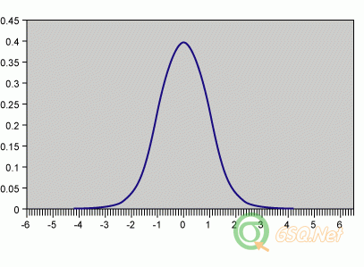
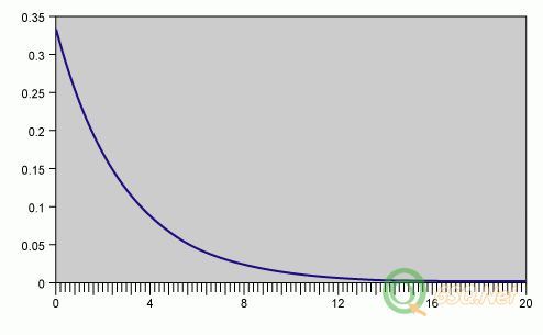
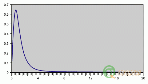
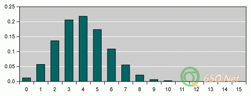
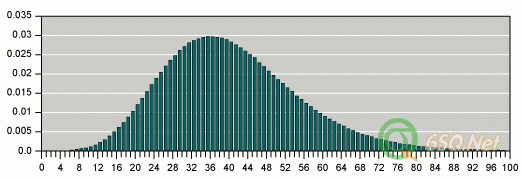
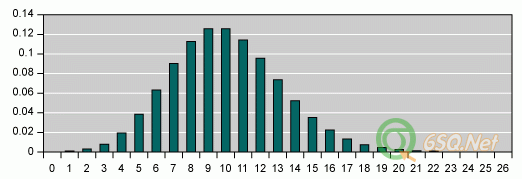
**Understanding Statistical Distributions for Six Sigma** To interpret data, consultants need to understand distributions. This article discusses how to understand different types of statistical distributions, understand the uses of different distributions, and make assumptions given a known distribution. By J. DeLayne Stroud Many consultants remember the hypothesis testing roadmap, which was a great template for deciding what type of test to perform. However, think about the type of data one gets. What if there is only summarized data? How can that data be used to make conclusions? Having the raw data is the best case scenario, but if it is not available, there are still tests that can be performed. In order to not only look at data, but also interpret it, consultants need to understand distributions. This article discusses how to: •Understand different types of statistical distributions. •Understand the uses of different distributions. •Make assumptions given a known distribution. Six Sigma Green Belts receive training focused on shape, center and spread. The concept of shape, however, is limited to just the normal distribution for continuous data. This article will expand upon the notion of shape, described by the distribution (for both the population and sample). **Getting Back to the Basics**With probability, statements are made about the chances that certain outcomes will occur, based on an assumed model. With statistics, observed data is used to determine a model that describes this data. This model relates to the distribution of the data. Statistics moves from the sample to the population while probability moves from the population to the sample. Inferential statistics is the science of describing population parameters based on sample data. Inferential statistics can be used to: •Establish a process capability (determine defects per million). •Utilize distributions to estimate the probability of a variable occurring given known parameters.Inferential statistics are based on a normal distribution. **Figure 1: Normal Curve and Probability Areas******Normal curve distribution can be expanded on to learn about other distributions. The appropriate distribution can be assigned based on an understanding of the process being studied in conjunction with the type of data being collected and the dispersion or shape of the distribution. It can assist with determining the best analysis to perform. **Types of Distributions**Distributions are classified in the same ways as data is classified - continuous and discrete: •Continuous probability distributions are probabilities associated with random variables that are able to assume any of an infinite number of values along an interval. •Discrete probability distributions are listings of all possible outcomes of an experiment, along with their respective probabilities of occurrence.**Distribution Descriptions**Probability mass function (pmf) - For discrete variables, the pmf is the probability that a variate takes the value x. Probability density function (pdf) - For continuous variables, the pdf is the probability that a variate assumes the value x, expressed in terms of an integral between two points. In the continuous sense, one cannot give a probability of a specific x on a continuum – it will be some specific (and small) range. For additional insight, think of **_x + _****_D_****_x_** where **_D_****_x_** is small. The notation for the pdf is f(x). For discrete distributions: f(x) = P(X = x) Some refer to this as the probability mass function, since it is evaluating the probability upon that one discrete mass. For continuous distributions, one mass cannot be established. Cumulative density function (cdf) - The probability that a variable takes a value less than or equal to x. **Figure 2: Normal Distribution Cdf**Cdf progresses to a value of 1 because there cannot be a probability greater than 1. Once again, cdf is F(x) = P(X < x). This holds for both continuous and discrete. **Parameters**Parameter is a population description. Consultants rely on parameters to characterize the distributions. There are three parameters: •Location parameter - the lower or midpoint (as prescribed by the distribution) of the range of the variate (think of the mean) •Scale parameter - determines the scale of measurement for x (magnitude of the x-axis scale) (think of the standard deviation) •Shape parameter - defines the pdf shape within a family of shapesNot all distributions have all the parameters. For example, the normal distribution parameters have just the mean and standard deviation. Just those two need to be known to describe a normal population. **Summary of Distributions**The remaining portion of this article will summarize the various shapes, basic assumptions and uses of distributions. Keep in mind that there is a different pdf and different distribution parameters associated with each. Normal Distribution (Gaussian Distribution) **Figure 3: Normal Distribution Shape**Basic assumptions: •Symmetrical distribution about the mean (bell-shaped curve). •Commonly used in inferential statistics. •Family of distributions characterized is by m and s.Uses include: •Probabilistic assessments of distribution of time between independent events occurring at a constant rate. •Mean is the inverse of the Poisson distribution. •Shape can be used to describe failure rates that are constant as a function of usage. **Exponential Distribution** **Figure 4:Exponential Distribution Shape**Basic assumptions: •Family of distributions characterized by its m. •Distribution of time between independent events occurring at a constant rate. •Mean is the inverse of the Poisson distribution. •Shape can be used to describe failure rates that are constant as a function of usage.Uses include probabilistic assessments of: •Mean time between failure (MTBF). •Arrival times. •Time, distance or space between occurrences of the events of interest. •Queuing or wait-line theories. **Lognormal Distribution** **Figure 5: Lognormal Distribution Shape**Basic assumptions: •Asymmetrical and positively skewed distribution that is constrained by zero. •Distribution can exhibit many pdf shapes. •Describes data that has a large range of values. •Can be characterized by m and s.Uses include simulations of: •Distribution of wealth. •Machine downtimes. •Duration of time. •Phenomenon that has a positive skew (tails to the right). **Weibull Distribution** **Figure 6: Weibull Distribution Pdf**Basic assumptions: •Family of distributions. •Can be used to describe many types of data. •Fits many common distributions (normal, exponential and lognormal). •The differing factors are the scale and shape parameters.Uses include: •Lifetime distributions. •Reliability applications. •Failure probabilities that vary over time. •Can describe burn-in, random, and wear-out phases of a life cycle (bathtub curve). **Binomial Distribution**** ****Figure 7: Binomial Distribution Shape**Basic assumptions: •Discrete distribution. •Number of trials are fixed in advance. •Just two outcomes for each trial. •Trials are independent. •All trials have the same probability of occurrence.Uses include: •Estimating the probabilities of an outcome in any set of success or failure trials. •Sampling for attributes (acceptance sampling). •Number of defective items in a batch size of n. •Number of items in a batch. •Number of items demanded from an inventory.**Geometric**** ****Figure 8: Geometric Distribution Pdf**Basic assumptions: •Discrete distribution. •Just two outcomes for each trial. •Trials are independent. •All trials have the same probability of occurrence. •Waiting time until the first occurrence.Uses include: •Number of failures before the first success in a sequence of trials with probability of success p for each trial. •Number of items inspected before finding the first defective item - for example, the number of interviews performed before finding the first acceptable candidate**Negative Binomial**** ****Figure 9: Negative Binomial Distribution Pdf**Basic assumptions: •Discrete distribution. •Predetermined number of occurrences - s. •Just two outcomes for each trial. •Trials are independent. •All trials have the same probability of occurrence.Uses include: •Number of failures before the sth success in a sequence of trials with probability of success p for each trial. •Number of good items inspected before finding the sth defective item.**Poisson Distribution**** ****Figure 10: Poisson Distribution Pdf**Basic assumptions: •Discrete distribution. •Length of the observation period (or area) is fixed in advance. •Events occurs at a constant average rate. •Occurrences are independent. •Rare event.Uses include: •Number of events in an interval of time (or area) when the events are occurring at a constant rate. •Number of items in a batch of random size. •Design reliability tests where the failure rate is considered to be constant as a function of usage.**Hypergeometric**Shape is similar to Binomial/Poisson distribution. Basic assumptions: •Discrete distribution. •Number of trials are fixed in advance. •Just two outcomes for each trial. •Trials are independent. •Sampling without replacement. •This is an exact distribution – the Binomial and Poisson are approximations to this.**Other Distributions**There are other distributions - for example, sampling distributions and X2, t and F distributions.
**Summary**Distribution refers to the behavior of a process described by plotting the number of times a variable displays a specific value or range of values rather than by plotting the value itself. It is often said that a picture is worth a thousand words. Viewing data graphically will make a much greater impact to an audience. Becoming familiar with the various distributions can help consultants to better interpret their data. **About the Author: **J. DeLayne Stroud is a Six Sigma Master Black Belt project manager with DeLeeuw Associates, a division of Conversion Services International. He retired from Bank of America in 2005 with more than 20 years of experience as an executive in project and change management in the banking industry. He has led multiple Design for Six Sigma and Lean initiatives. During his career, Mr. Stroud was a senior project manager in some of the largest mergers and change initiatives in the history of the financial services industry, including former banks such as General Bancshares, Boatmen's Bank, Centerre Bank, Barnett Bank and BankAmerica. He can be reached at jstroud@deleeuwinc.com .
没有找到相关结果
已邀请:





4 个回复
wulh (威望:0) (上海 徐汇区) 航空相关 员工
赞同来自: